Dynamic Time Warping

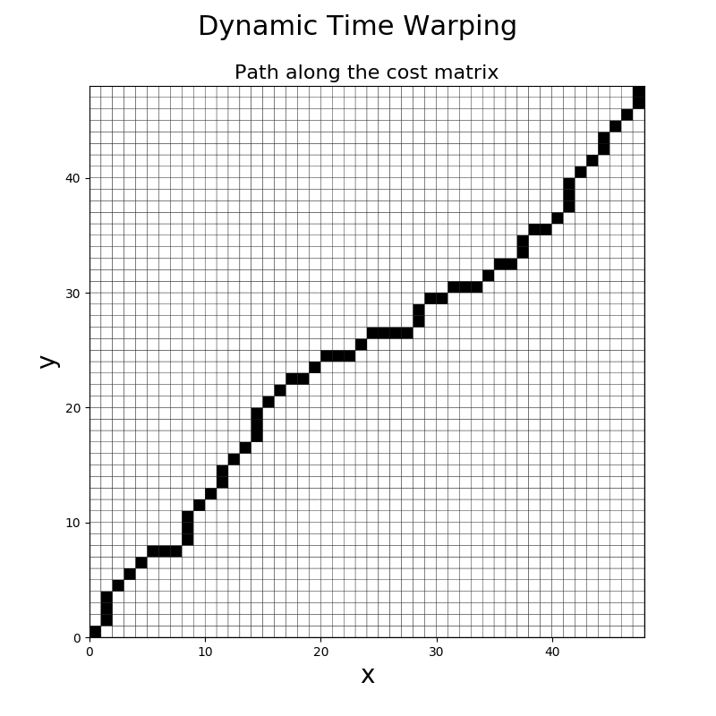
This example shows how to compute and visualize the optimal path when computing the Dynamic Time Warping distance between two time series. It is implemented as pyts.utils.dtw().

import numpy as np
import matplotlib.pyplot as plt
from pyts.utils import dtw

# Parameters
n_samples, n_features = 2, 48

# Toy dataset
rng = np.random.RandomState(41)
x, y = rng.randn(n_samples, n_features)

# Dynamic Time Warping
D, path = dtw(x, y, dist='absolute', return_path=True)

# Visualize the result
timestamps = np.arange(n_features + 1)
matrix = np.zeros([n_features + 1, n_features + 1])
for i in range(len(path)):
    matrix[path[i][0], path[i][1]] = 1

plt.figure(figsize=(8, 8))
plt.pcolor(timestamps, timestamps, matrix, edgecolors='k', cmap='Greys')
plt.xlabel('x', fontsize=20)
plt.ylabel('y', fontsize=20)
plt.title("Path along the cost matrix", fontsize=16)
plt.suptitle("Dynamic Time Warping", fontsize=22)
plt.show()

Total running time of the script: ( 0 minutes 0.200 seconds)