SAXVSM

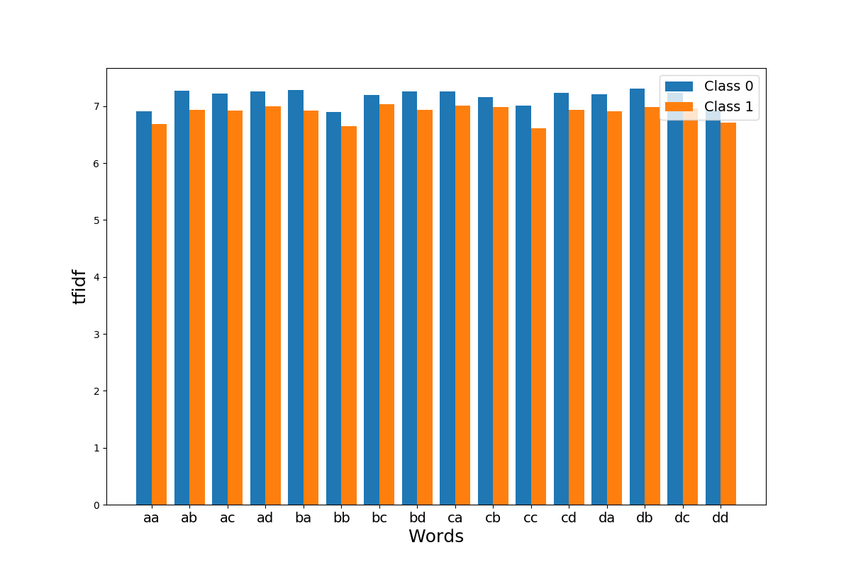
This example shows how the SAXVSM algorithm transforms a dataset consisting of time series and their corresponding labels into a document-term matrix using tfidf. Each class is represented as a tfidf vector. For an unlabeled time series, the predicted label is the label of the tfidf vector giving the highest cosine similarity with the tf vector of the unlabeled time series. Here we plot the tfidf vectors for each clss. SAXVSM algorithm is implemented as pyts.classification.SAXVSMClassifier.

import numpy as np
import matplotlib.pyplot as plt
from pyts.classification import SAXVSMClassifier

# Parameters
n_samples, n_features = 100, 144
n_classes = 2

# Toy dataset
rng = np.random.RandomState(41)
X = rng.randn(n_samples, n_features)
y = rng.randint(n_classes, size=n_samples)

# SAXVSM transformation
saxvsm = SAXVSMClassifier(window_size=2, sublinear_tf=True)
saxvsm.fit(X, y)
tfidf = saxvsm.tfidf_.toarray()

# Visualize the transformation
plt.figure(figsize=(12, 8))
plt.bar(np.arange(tfidf[0].size) - 0.2, tfidf[0], width=0.4, label='Class 0')
plt.bar(np.arange(tfidf[0].size) + 0.2, tfidf[1], width=0.4, label='Class 1')
plt.xticks(np.arange(tfidf[0].size),
           np.vectorize(saxvsm.vocabulary_.get)(np.arange(tfidf[0].size)),
           fontsize=14)
plt.xlabel("Words", fontsize=18)
plt.ylabel("tfidf", fontsize=18)
plt.legend(loc='best', fontsize=14)
plt.show()

Total running time of the script: ( 0 minutes 0.213 seconds)