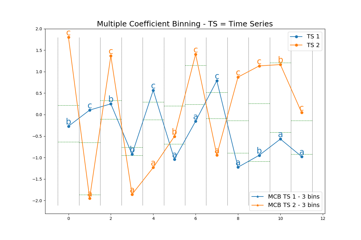
Multiple Coefficient Binning

This example shows how the MCB algorithm transforms a dataset of time series of real numbers into a list of sequences of letters. It is implemented as pyts.quantization.MCB.

import numpy as np
import matplotlib.lines as mlines
import matplotlib.pyplot as plt
from pyts.quantization import MCB

# Parameters
n_samples, n_features = 6, 12

# Toy dataset
rng = np.random.RandomState(41)
X = rng.randn(n_samples, n_features)

# MCB transformation
n_bins = 3
quantiles = 'empirical'
mcb = MCB(n_bins=n_bins, quantiles=quantiles)
X_mcb = mcb.fit_transform(X)

# Compute bins
bins = mcb._bins

# Show the results for the first time series
plt.figure(figsize=(12, 8))
# First time series
plt.plot(X[0], 'o-', label='TS 1')
for x, y, s in zip(range(n_features), X[0], X_mcb[0]):
    plt.text(x, y, s, ha='center', va='bottom', fontsize=20, color='#1f77b4')
# Second time series
plt.plot(X[5], 'o-', label='TS 2')
for x, y, s in zip(range(n_features), X[5], X_mcb[5]):
    plt.text(x, y, s, ha='center', va='bottom', fontsize=20, color='#ff7f0e')
plt.hlines(bins, np.arange(n_features) - 0.5, np.arange(n_features) + 0.5,
           color='g', linestyles='--', linewidth=0.7)
plt.vlines(np.arange(n_features + 1) - 0.5, X.min(), X.max(),
           linestyles='--', linewidth=0.5)
mcb_legend_1 = mlines.Line2D([], [], color='#1f77b4', marker='*',
                             label='MCB TS 1 - {0} bins'.format(n_bins))
mcb_legend_2 = mlines.Line2D([], [], color='#ff7f0e', marker='*',
                             label='MCB TS 2 - {0} bins'.format(n_bins))
first_legend = plt.legend(handles=[mcb_legend_1, mcb_legend_2],
                          fontsize=14, loc=4)
ax = plt.gca().add_artist(first_legend)
plt.legend(loc='best', fontsize=14)
plt.title("Multiple Coefficient Binning - TS = Time Series", fontsize=18)
plt.show()

Total running time of the script: ( 0 minutes 0.043 seconds)