Discrete Fourier Transform

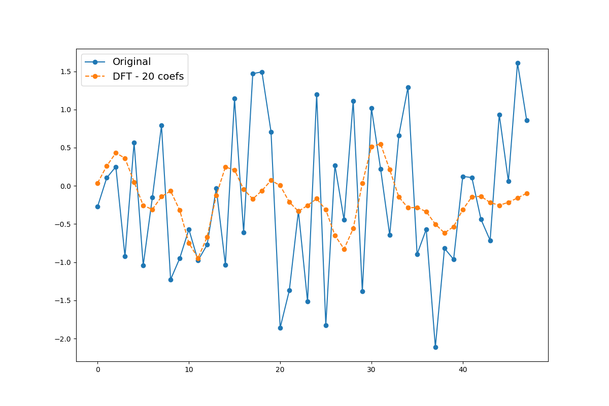
This example shows how you can approximate a time series using only some of its Fourier coefficients using pyts.approximation.DFT.

import numpy as np
import matplotlib.pyplot as plt
from pyts.approximation import DFT

# Parameters
n_samples, n_features = 100, 48

# Toy dataset
rng = np.random.RandomState(41)
X = rng.randn(n_samples, n_features)

# DFT transformation
n_coefs = 20
norm_mean = False
norm_std = False
dft = DFT(n_coefs=n_coefs, norm_mean=norm_mean, norm_std=norm_std)
X_dft = dft.fit_transform(X)

# Compute the approximation for the first time series
timestamps = np.arange(n_features) / n_features
x_dft = np.zeros(n_features)
for n in range(n_coefs // 2):
    x_dft += X_dft[0, 2 * n] * np.cos(2 * n * np.pi * timestamps) / n_features
    x_dft += X_dft[0, (2 * n) + 1] * np.sin(2 * n * np.pi * timestamps) / \
        n_features

# Show the results for the first time series
plt.figure(figsize=(12, 8))
plt.plot(X[0], 'o-', label='Original')
plt.plot(x_dft, 'o--', label='DFT - {0} coefs'.format(n_coefs))
plt.legend(loc='best', fontsize=14)
plt.show()

Total running time of the script: ( 0 minutes 0.024 seconds)